
Face Recognition - LBPH Algorithm
Human beings perform face recognition automatically every day and practically with no effort.
Although it sounds like a very simple task for us, it has proven to be a complex task for a computer, as it has many variables that can impair the accuracy of the methods, for example: illumination variation, low resolution, occlusion, amongst other.
In computer science, face recognition is basically the task of recognizing a person based on its facial image. It has become very popular in the last two decades, mainly because of the new methods developed and the high quality of the current videos/cameras.
Note that face recognition is different of face detection:
-
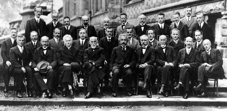
Face Detection: it has the objective of finding the faces (location and size) in an image and probably extract them to be used by the face recognition algorithm.
-
Face Recognition: with the facial images already extracted, cropped, resized and usually converted to grayscale, the face recognition algorithm is responsible for finding characteristics which best describe the image.
The face recognition systems can operate basically in two modes:
-
Verification or authentication of a facial image: it basically compares the input facial image with the facial image related to the user which is requiring the authentication. It is basically a 1x1 comparison.
-
Identification or facial recognition: it basically compares the input facial image with all facial images from a dataset with the aim to find the user that matches that face. It is basically a 1xN comparison.
There are different types of face recognition algorithms, for example:
-
Eigenfaces (1991)
-
Fisherfaces (1997)
Each method has a different approach to extract the image information and perform the matching with the input image. However, the methods Eigenfaces and Fisherfaces have a similar approach as well as the SIFT and SURF methods.
Today we gonna talk about one of the oldest (not the oldest one) and more popular face recognition algorithms: Local Binary Patterns Histograms (LBPH).
Objective
The objective of this post is to explain the LBPH as simple as possible, showing the method step-by-step.
As it is one of the easier face recognition algorithms I think everyone can understand it without major difficulties.
Introduction
Local Binary Pattern (LBP) is a simple yet very efficient texture operator which labels the pixels of an image by thresholding the neighborhood of each pixel and considers the result as a binary number.
It was first described in 1994 (LBP) and has since been found to be a powerful feature for texture classification. It has further been determined that when LBP is combined with histograms of oriented gradients (HOG) descriptor, it improves the detection performance considerably on some datasets.
Using the LBP combined with histograms we can represent the face images with a simple data vector.
As LBP is a visual descriptor it can also be used for face recognition tasks, as can be seen in the following step-by-step explanation.
Note: you can read more about the LBPH here: http://www.scholarpedia.org/article/Local_Binary_Patterns
Step-by-Step
Now that we know a little more about face recognition and the LBPH, let’s go further and see the steps of the algorithm:
- Parameters: the LBPH uses 4 parameters:
-
Radius: the radius is used to build the circular local binary pattern and represents the radius around the central pixel. It is usually set to 1.
-
Neighbors: the number of sample points to build the circular local binary pattern. Keep in mind: the more sample points you include, the higher the computational cost. It is usually set to 8.
-
Grid X: the number of cells in the horizontal direction. The more cells, the finer the grid, the higher the dimensionality of the resulting feature vector. It is usually set to 8.
-
Grid Y: the number of cells in the vertical direction. The more cells, the finer the grid, the higher the dimensionality of the resulting feature vector. It is usually set to 8.
Don’t worry about the parameters right now, you will understand them after reading the next steps.
2. Training the Algorithm: First, we need to train the algorithm. To do so, we need to use a dataset with the facial images of the people we want to recognize. We need to also set an ID (it may be a number or the name of the person) for each image, so the algorithm will use this information to recognize an input image and give you an output. Images of the same person must have the same ID. With the training set already constructed, let’s see the LBPH computational steps.
3. Applying the LBP operation: The first computational step of the LBPH is to create an intermediate image that describes the original image in a better way, by highlighting the facial characteristics. To do so, the algorithm uses a concept of a sliding window, based on the parameters radius and neighbors.
The image below shows this procedure:
Based on the image above, let’s break it into several small steps so we can understand it easily:
-
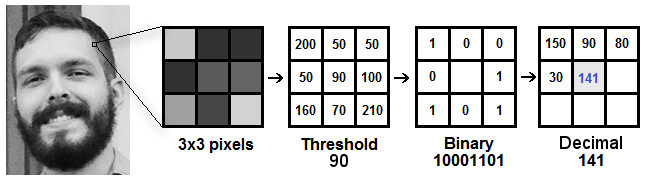
Suppose we have a facial image in grayscale.
-
We can get part of this image as a window of 3x3 pixels.
-
It can also be represented as a 3x3 matrix containing the intensity of each pixel (0~255).
-
Then, we need to take the central value of the matrix to be used as the threshold.
-
This value will be used to define the new values from the 8 neighbors.
-
For each neighbor of the central value (threshold), we set a new binary value. We set 1 for values equal or higher than the threshold and 0 for values lower than the threshold.
-
Now, the matrix will contain only binary values (ignoring the central value). We need to concatenate each binary value from each position from the matrix line by line into a new binary value (e.g. 10001101). Note: some authors use other approaches to concatenate the binary values (e.g. clockwise direction), but the final result will be the same.
-
Then, we convert this binary value to a decimal value and set it to the central value of the matrix, which is actually a pixel from the original image.
-
At the end of this procedure (LBP procedure), we have a new image which represents better the characteristics of the original image.
-
Note: The LBP procedure was expanded to use a different number of radius and neighbors, it is called Circular LBP.
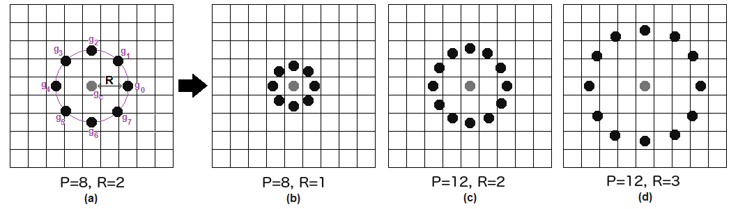
It can be done by using bilinear interpolation. If some data point is between the pixels, it uses the values from the 4 nearest pixels (2x2) to estimate the value of the new data point.
4. Extracting the Histograms: Now, using the image generated in the last step, we can use the Grid X and Grid Y parameters to divide the image into multiple grids, as can be seen in the following image:
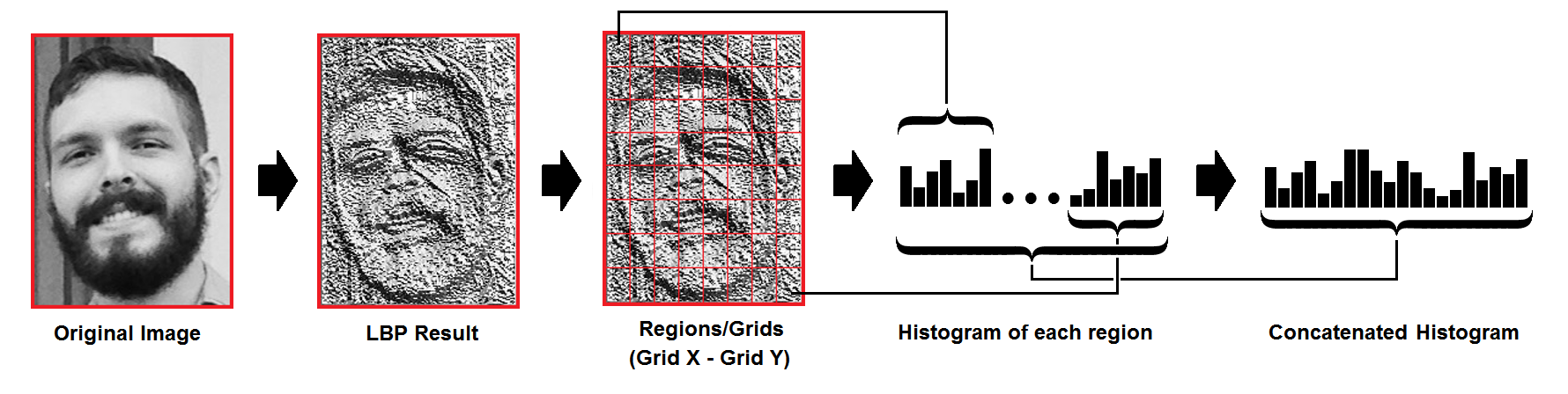
Based on the image above, we can extract the histogram of each region as follows:
-
As we have an image in grayscale, each histogram (from each grid) will contain only 256 positions (0~255) representing the occurrences of each pixel intensity.
-
Then, we need to concatenate each histogram to create a new and bigger histogram. Supposing we have 8x8 grids, we will have 8x8x256=16.384 positions in the final histogram. The final histogram represents the characteristics of the image original image.
The LBPH algorithm is pretty much it.
5. Performing the face recognition: In this step, the algorithm is already trained. Each histogram created is used to represent each image from the training dataset. So, given an input image, we perform the steps again for this new image and creates a histogram which represents the image.
-
So to find the image that matches the input image we just need to compare two histograms and return the image with the closest histogram.
-
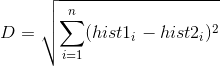
We can use various approaches to compare the histograms (calculate the distance between two histograms), for example: euclidean distance, chi-square, absolute value, etc. In this example, we can use the Euclidean distance (which is quite known) based on the following formula:
-
So the algorithm output is the ID from the image with the closest histogram. The algorithm should also return the calculated distance, which can be used as a ‘confidence’ measurement. Note: don’t be fooled about the ‘confidence’ name, as lower confidences are better because it means the distance between the two histograms is closer.
-
We can then use a threshold and the ‘confidence’ to automatically estimate if the algorithm has correctly recognized the image. We can assume that the algorithm has successfully recognized if the confidence is lower than the threshold defined.
Conclusions
-
LBPH is one of the easiest face recognition algorithms.
-
It can represent local features in the images.
-
It is possible to get great results (mainly in a controlled environment).
-
It is robust against monotonic gray scale transformations.
-
It is provided by the OpenCV library (Open Source Computer Vision Library).
LBPH algorithm
I am implementing the LBPH algorithm in Go programming language. The project is available on Github and is distributed under the MIT license, so feel free to contribute to the project (any contributions are welcome). Link to the project: https://github.com/kelvins/lbph
Note: as mentioned in the conclusions, the LBPH is also provided by the OpenCV library. The OpenCV library can be used by many programming languages (e.g. C++, Python, Ruby, Matlab).
If you liked this story please give it a clap. It motivates me to write more stories about face recognition.
References
-
Ahonen, Timo, Abdenour Hadid, and Matti Pietikainen. “Face description with local binary patterns: Application to face recognition.” IEEE transactions on pattern analysis and machine intelligence 28.12 (2006): 2037–2041.
-
Ojala, Timo, Matti Pietikainen, and Topi Maenpaa. “Multiresolution gray-scale and rotation invariant texture classification with local binary patterns.” IEEE Transactions on pattern analysis and machine intelligence 24.7 (2002): 971–987.
-
Ahonen, Timo, Abdenour Hadid, and Matti Pietikäinen. “Face recognition with local binary patterns.” Computer vision-eccv 2004 (2004): 469–481.
-
LBPH OpenCV: https://docs.opencv.org/2.4/modules/contrib/doc/facerec/facerec_tutorial.html#local-binary-patterns-histograms
-
Local Binary Patterns: http://www.scholarpedia.org/article/Local_Binary_Patterns